Mathematics and the Real World (33 page)

The search for methods of calculating probabilities in situations with incomplete information at the outset, a subject raised by Jacob Bernoulli, led to the development of a technique based on a mathematical theorem known as the
central limit theorem
. The first move in that direction was made by the French mathematician Abraham de Moivre (1667–1754). He spent many years in England, much of the time with Newton, after being exiled there as a result of the persecution of the Huguenots in France. Whereas Jacob Bernoulli examined the extent of the deviations of the average from expectation and showed that most of the deviations are concentrated around zero, de Moivre decided to study the distribution of those deviations, in other words, how they divide between relatively large deviations and medium and small ones. He focused on Bernoulli's coin tossing experiments in which, let us say, heads gives a prize of one, and tails yields nothing. He found, using a mathematical calculation, that if the size of the deviation from the average is divided by the square root of the number of throws (i.e., instead of dividing the total winnings by
n
after
n
flips
of the coin to find the deviation from expectation, he divided by √
n
), the distribution becomes closer and closer to a bell shape. If the coin is not equally balanced, with the chance of heads say
a
, the shape of the bell will depend on the value of
a
, but if the result is divided by √
a
(1 –
a
), which in due course came to be known as the standard deviation, the distribution obtained is bell shaped independent of the value of
a
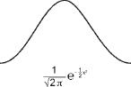
. De Moivre actually calculated the shape of the bell obtained, shown in the diagram together with the formula (which is unimportant for our current purposes).

It is not clear whether de Moivre realized the implications of his discovery for the theory of statistics and its practice, but several famous mathematicians generalized de Moivre's limit law and found that it applies far more widely. The research reached its pinnacle in the work by Pierre-Simon Laplace (1749–1827), who as well as proving the wider applicability of the central limit theorem also laid the foundations for its uses in statistical analyses. Laplace was born in Normandy, France, and his family intended that he become a priest, but his mathematical inclinations prevailed, and he was accepted to carry out research under D’Alembert. He completed a research project in mechanics, a study that earned him a position in the military academy as a mathematics teacher and an artillery officer. There he befriended Napoleon Bonaparte, a friendship that certainly did him no harm in the politically stormy atmosphere in France at that time. He survived the French Revolution by maintaining a low profile and even became head of the French Academy. His book on the analytical theory of probability, published in 1812, he dedicated to Napoleon.

At about the same time, in a book published in 1810, Gauss himself presented the same limit law. Gauss, who clearly was familiar with de Moivre's work, focused his attention on a different aspect than did Laplace.
Gauss was very interested in the results of measurements and in the question of how to find the closest value to the correct one in measurements that include random measurement errors. With that in mind, Gauss developed a system that still today is called the least-squares method, and, based on the assumption that the errors in the calculations are random and independent, showed that the average was the value that predicted the correct value with the greatest degree of accuracy. He extended the system to more complex calculations and, in that framework, even proved the central limit theorem. The bell-shaped distribution is today called the normal distribution and also the Gaussian distribution, in recognition of his contribution.

Laplace and Gauss, as well as many of their research colleagues, realized that the statistical methods could be used to answer questions beyond the field of gambling and flipping coins. If a particular outcome is the result of many occurrences that include randomness and those random occurrences are independent, the distribution of the outcomes will be similar to the normal distribution around the average value of the outcome. Laplace, who was also interested in and contributed much to astronomy, used this technique to analyze deviations of the planes of orbit of the planets from one, middle, plane. The planes of orbit of the planets around the Sun almost coincide, and their deviations from one middle plane are very small. Are those deviations random, or do they have another cause? By using the statistical technique he had developed, Laplace showed that the deviations are a close approximation to the expected distribution based on the central limit law, and therefore it was highly probable that they were random deviations from one orbit plane. The expression “highly probable” is an indication that this is a statistical result and not a mathematical certainty. At the same time Laplace showed that the planes of orbit of the various comets do not comply with the expectation based on the central limit law, and he therefore concluded that those deviations were not caused by random deviations from one plane. Gauss also used the least-squares method for calculations in astronomy. At that time the asteroid Ceres, which moved on an orbit that disappeared behind the Sun, was identified, and the question was when would it reappear on the other side of the Sun. Little data had been calculated regarding its path, and what there was included many measurement
errors. Gauss applied his method and predicted with surprising accuracy Ceres's continued route, a prediction that justifiably brought him worldwide renown.

The work of Gauss and Laplace brought the mathematics of randomness and its uses in statistics to a center-stage position in science. Since then, the central limit law has been found to be correct, with minor changes, in more general cases than those analyzed by Laplace and Gauss. Especially worthy of mention are the Russian mathematician Pafnuty Chebyshev and his students Andrei Markov and Aleksandr Lyapunov. They were active in the second half of the nineteenth century and firmly established the central limit theorem without the assumption that the random events that lead to deviations from the average have equal distributions, that is, they have the same characteristics of randomness. Such a general rule was important to justify its uses for situations that appear in nature. The lack of interdependence in nature between the random events can be justified, but it is more difficult to justify the assumption that the random characteristics are equal for all events. The work of the Russian mathematicians reduced the gap between the mathematical theorem and its possible applications, and thus the central limit theorem, together with other limit theorems, became the norm for the various uses of statistics.

The main use of limit theorems is to estimate statistical values such as the average, the dispersion, and so on, of data that have random inaccuracy. It is generally difficult to assess whether the errors are random or not. Even if the errors are random, however, absorbing and understanding the technique required for the use of the mathematics that developed involves difficulties that can themselves cause errors. Again, the difficulties derive from the way our intuition relates to data. We will mention two such difficulties.

We are exposed to huge numbers of statistical surveys in our day-to-day lives. When the results of a survey are published, it is usually done in the following form: The survey found that (say) 47 percent of the voters intend to vote for a particular candidate, with a survey error of plus or minus 2 percent. Yet only part of the conditions and reservations about the results are presented in the survey report. In effect, the correct conclusion
from the survey would be that there is a 95 percent chance that the proportion of voters who intend to support that particular candidate is between 47 percent plus 2 percent and 47 percent minus 2 percent. The 95 percent bound is quite normal in practice in statistics. The survey can be devised such that the chance that the assessment derived from the survey is correct is 99 percent (it will then cost more to carry out the survey), or any other number less than a hundred. The condition of 95 or 99 percent is not published. Why not? The fact that the declared limits of the results, that is, that the resulting interval of 45 to 49 percent, applies with only a 95 percent probability could have great importance. The reason would seem to be the difficulty in absorbing quantifications.

There is another aspect of statistical samples that is difficult to understand. Let us say that we are told that a survey of five hundred people selected at random in Israel is sufficient to ensure a result with a plus or minus 2 percent survey error (with 95 percent accuracy). The population of Israel is about eight million. What size sample would be required to achieve that level of confidence in the United States with 320 million inhabitants? Would it need to be forty times the sample size in Israel? Most people asked that question would answer intuitively that a much larger sample is needed in the United States than in Israel. The right answer is that the same size sample is required in both cases. The size of the sampled population affects only the difficulty of selecting the sample randomly. Once we have sampled correctly (and most survey failures derive from the inability to sample correctly), the size of the survey error is determined only by the size of the sample. This is another example of the discrepancy between human intuition and mathematical results. Evolution indeed did not prepare us for large samples.

40. THE MATHEMATICS OF LEARNING FROM EXPERIENCE

Let us go back to a development that started in the eighteenth century that had an aura of logic about it and is therefore “responsible” for serious
errors in the application of the theory. The statistical methods described in the previous section help us when the particular probabilities are known, and we need only to calculate the chance of a specific event occurring or, when it is possible, to estimate the statistical parameters. The technique does not teach us how to improve the assessments when new information is supplied to us. It was de Moivre, in his book on methods of dealing with randomness, who asked the question of how to act when new information is added. It was Thomas Bayes who answered the question, and the system whose fundamentals he put forward is known as the Bayesian method.

Thomas Bayes (1702–1761) was born in England but studied mathematics and theology at the University of Edinburgh, Scotland. He was more interested in theology and, following in the footsteps of his father, who was a Presbyterian minister in London, served in a similar capacity in the Mount Zion Chapel in Tunbridge Wells, Kent, England. In his lifetime he published only two works. One was on religious matters. The other was an attempt to defend Newton's approach to infinitesimal calculus against the severe attacks that claimed that fluxion had no logical basis. The criticism was published by the famous Irish philosopher Bishop George Berkeley (after whom the University of California, Berkeley, is named). Bayes did not see it fit to publish his formula in his lifetime, and it was published only after his death by his friend Richard Price, who was bequeathed Bayes's writings, and who realized the importance of that work.

Bayes's formula is very easy to understand technically but is also very difficult to absorb and apply intuitively. We will discuss the reasons for this and its sometimes-serious results in the coming sections. Here we will just present and explain the Bayesian formula itself (the calculations can be skipped without disturbing the overall picture).

We will start with an example based on a question that was asked in the school matriculation examination in probability in Israel in 2010. Of three boxes, the first contains two silver coins, the second has one silver coin and one gold coin, and the third holds two gold coins. One of the boxes is chosen at random, and one of the coins in it is chosen at random. The simple question is, what are the chances that the coin left in the box is a silver one? For reasons of symmetry one could conclude that the chance is 50 percent because the question does not differentiate between the roles of the two types of coin. That was the answer that would have been given before the revolution of Fermat and Pascal (without using the concept of “chance,” which did not exist then). One can also carry out the following calculation: Each box has a probability of one-third of being selected. If the first is chosen, the probability of the coin that is left in the box being silver is one (i.e., a certainty). If the second box is chosen and one coin is chosen randomly, the chances that the one left is silver is one-half. If the third box is chosen, the remaining coin after the choice of one is not silver. Now calculate
, and we obtain that the chance is 50 percent.