Data Mining (76 page)
Authors: Mehmed Kantardzic

Figure 9.8.
Dendrogram by complete-link method for the data set in Figure
9.6
.
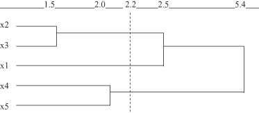
Selecting, for example, a threshold measure of similarity s = 2.2, we can recognize from the dendograms in Figures
9.7
and
9.8
that the final clusters for single-link and complete-link algorithms are not the same. A single-link algorithm creates only two clusters: {x
1
, x
2
, x
3
} and {x
4
, x
5
}, while a complete-link algorithm creates three clusters: {x
1
}, {x
2
, x
3
}, and {x
4
, x
5
}.
Unlike traditional agglomerative methods,
Chameleon
is a clustering algorithm that tries to improve the clustering quality by using a more elaborate criterion when merging two clusters. Two clusters will be merged if the interconnectivity and closeness of the merged clusters is very similar to the interconnectivity and closeness of the two individual clusters before merging.
To form the initial subclusters, Chameleon first creates a graph G = (V, E), where each node v ∈ V represents a data sample, and a weighted edge e(v
i
, v
j
) exists between two nodes v
i
and v
j
if v
j
is one of the k-nearest neighbors of v
i
. The weight of each edge in G represents the closeness between two samples, that is, an edge will weigh more if the two data samples are closer to each other.
Chameleon
then uses a graph-partition algorithm to recursively partition G into many small, unconnected subgraphs by doing a min-cut on G at each level of recursion. Here, a min-cut on a graph G refers to a partitioning of G into two parts of close, equal size such that the total weight of the edges being cut is minimized. Each subgraph is then treated as an initial subcluster, and the algorithm is repeated until a certain criterion is reached.
In the second phase, the algorithm goes bottom-up.
Chameleon
determines the similarity between each pair of elementary clusters C
i
and C
j
according to their relative interconnectivity
RI
(C
i
, C
j
) and their relative closeness
RC
(C
i
, C
j
). Given that the interconnectivity of a cluster is defined as the total weight of edges that are removed when a min-cut is performed, the relative interconnectivity
RI
(C
i
, C
j
) is defined as the ratio between the interconnectivity of the merged cluster C
i
and C
j
to the average interconnectivity of C
i
and C
j
. Similarly, the relative closeness
RC
(C
i
, C
j
) is defined as the ratio between the closeness of the merged cluster of C
i
and C
j
to the average internal closeness of C
i
and C
j
. Here the closeness of a cluster refers to the average weight of the edges that are removed when a min-cut is performed on the cluster.
The similarity function is then computed as a product:
RC
(C
i
, C
j
) *
RI
(C
i
, C
j
)
α
where α is a parameter between 0 and 1. A value of 1 for α will give equal weight to both measures while decreasing α will place more emphasis on
RI
(C
i
, C
j
). Chameleon can automatically adapt to the internal characteristics of the clusters and it is effective in discovering arbitrarily shaped clusters of varying density. However, the algorithm is not effective for high-dimensional data having O(n
2
) time complexity for n samples.
9.4 PARTITIONAL CLUSTERING
Every partitional-clustering algorithm obtains a single partition of the data instead of the clustering structure, such as a dendrogram, produced by a hierarchical technique. Partitional methods have the advantage in applications involving large data sets for which the construction of a dendrogram is computationally very complex. The partitional techniques usually produce clusters by optimizing a criterion function defined either locally (on a subset of samples) or globally (defined over all of the samples). Thus, we say that a clustering criterion can be either global or local. A global criterion, such as the Euclidean square-error measure, represents each cluster by a prototype or centroid and assigns the samples to clusters according to the most similar prototypes. A local criterion, such as the minimal MND, forms clusters by utilizing the local structure or context in the data. Therefore, identifying high-density regions in the data space is a basic criterion for forming clusters.
The most commonly used partitional-clustering strategy is based on the square-error criterion. The general objective is to obtain the partition that, for a fixed number of clusters, minimizes the total square-error. Suppose that the given set of N samples in an n-dimensional space has somehow been partitioned into K clusters {C
1
, C
2
, … , C
k
}. Each C
k
has n
k
samples and each sample is in exactly one cluster, so that Σn
k
= N, where k = 1, … , K. The mean vector M
k
of cluster C
k
is defined as the
centroid
of the cluster or
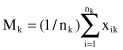
where x
ik
is the i
th
sample belonging to cluster C
k
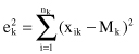
. The square-error for cluster C
k
is the sum of the squared Euclidean distances between each sample in C
k
and its centroid. This error is also called the
within-cluster variation
:
The square-error for the entire clustering space containing K clusters is the sum of the within-cluster variations:

The objective of a square-error clustering method is to find a partition containing K clusters that minimize for a given K.
The
K-means partitional-clustering algorithm
is the simplest and most commonly used algorithm employing a square-error criterion. It starts with a random, initial partition and keeps reassigning the samples to clusters, based on the similarity between samples and clusters, until a convergence criterion is met. Typically, this criterion is met when there is no reassignment of any sample from one cluster to another that will cause a decrease of the total squared error. K-means algorithm is popular because it is easy to implement, and its time and space complexity is relatively small. A major problem with this algorithm is that it is sensitive to the selection of the initial partition and may converge to a local minimum of the criterion function if the initial partition is not properly chosen.
The simple K-means partitional-clustering algorithm is computationally efficient and gives surprisingly good results if the clusters are compact, hyperspherical in shape, and well separated in the feature space. The basic steps of the K-means algorithm are
1.
select an initial partition with K clusters containing randomly chosen samples, and compute the centroids of the clusters;
2.
generate a new partition by assigning each sample to the closest cluster center;
3.
compute new cluster centers as the centroids of the clusters; and
4.
repeat steps 2 and 3 until an optimum value of the criterion function is found (or until the cluster membership stabilizes).
Let us analyze the steps of the K-means algorithm on the simple data set given in Figure
9.6
. Suppose that the required number of clusters is two, and initially, clusters are formed from a random distribution of samples: C
1
= {x
1
, x
2
, x
4
} and C
2
= {x
3
, x
5
}. The centriods for these two clusters are
