Data Mining (80 page)

Ideally, we would have to know the appropriate parameters ε and m of each cluster. But there is no easy way to get this information in advance for all clusters of the database. Therefore, DBSCAN uses global values for ε and m, that is, the same values for all clusters. Also, numerous experiments indicate that DBSCAN clusters for m > 4 do not significantly differ from the case m = 4, while the algorithm needs considerably more computations. Therefore, in practice we may eliminate the parameter m by setting it to four for low-dimensional databases. The main steps of DBSCAN algorithm are as follows:

• Arbitrarily select a point
  p
  .
  
• Retrieve all points density-reachable from
  p
  with respect to ε and m.
  
• If
  p
  is a core point, a new cluster is formed or existing cluster is extended.
  
• If
  p
  is a border point, no points are density-reachable from
  p
  , and DBSCAN visits the next point of the database.
  
• Continue the process with other points in the database until all of the points have been processed.
  
• Since global values for ε and m are used, DBSCAN may merge two clusters into one cluster, if two clusters of different density are “close” to each other. The are close if the distance between clusters is lower than ε.
  

Examples of clusters obtained by DBSCAN algorithm are illustrated in Figure
9.11
. Obviously, DBSCAN finds all clusters properly, independent of the size, shape, and location of clusters to each other.

Figure 9.11.
DBSCAN builds clusters of different shapes.

The main advantages of the DBSCAN clustering algorithm are as follows:

DBSCAN also has some disadvantages. The complexity of the algorithm is still very high, although with some indexing structures it reaches O (n × log n). Finding neighbors is an operation based on distance, generally the Euclidean distance, and the algorithm may find the curse of dimensionality problem for high-dimensional data sets. Therefore, most applications of the algorithm are for low-dimensional real-world data.

9.7 BIRCH ALGORITHM

BIRCH is an efficient clustering technique for data in Euclidean vector spaces. The algorithm can efficiently cluster data with a single pass, and also it can deal effectively with outliers. BIRCH is based on the notion of a
CF
and a
CF tree
.

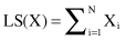
CF is a small representation of an underlying cluster that consists of one or many samples. BIRCH builds on the idea that samples that are close enough should always be considered as a group. CFs provide this level of abstraction with corresponding summarization of samples in a cluster. The idea is that a cluster of data samples can be represented by a triple of numbers (N, LS, SS), where N is the number of samples in the cluster, LS is the linear sum of the data points (vectors representing samples), and SS is the sum of squares of the data points. More formally, the component of vectors LS and SS are computed for every attribute X of data samples in a cluster:

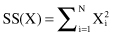
In Figure
9.12
five 2-D samples are representing the cluster, and their CF summary is given with components: N = 5, LS = (16, 30), and SS = (54, 190). These are common statistical quantities, and a number of different cluster characteristics and intercluster distance measures can be derived from them. For example, we can compute the centroid for the cluster based on its CF representation, without revisiting original samples. Coordinates of the centroid are obtained by dividing the components of the LS vector by N. In our example the centroid will have the coordinates (3.2, 6.0). The reader may check on the graphical interpretation of the data (Fig.
9.12
) that the position of the centroid is correct. The obtained summaries are then used instead of the original data for further clustering or manipulations with clusters. For example, if CF
₁
= (N
₁
, LS
₁
, SS
₁
) and CF
₂
= (N
₂
, LS
₂
, SS
₂
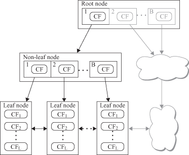
) are the CF entries of two disjoint clusters, then the CF entry of the cluster formed by merging the two clusters is

Figure 9.12.
CF representation and visualization for a 2-D cluster.

This simple equation shows us how simple the procedure is for merging clusters based on their simplified CF descriptions. That allows efficient incremental merging of clusters even for the streaming data.

BIRCH uses a hierarchical data structure called a CF tree for partitioning the incoming data points in an incremental and dynamic way. A CF tree is a height-balanced tree usually stored in a central memory. This allows fast lookups even when large data sets have been read. It is based on two parameters for nodes. CF nodes can have at maximum
B
children for non-leaf nodes, and a maximum of
L
entries for leaf nodes. Also, T is the threshold for the maximum diameter of an entry in the cluster. The CF tree size is a function of T. The bigger T is, the smaller the tree will be.

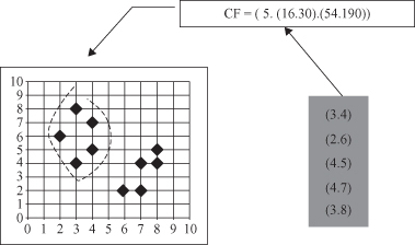
A CF tree (Fig
9.13
) is built as the data sample is scanned. At every level of the tree a new data sample is inserted to the closest node. Upon reaching a leaf, the sample is inserted to the closest CF entry, as long as it is not overcrowded (diameter of the cluster D > T after the insert). Otherwise, a new CF entry is constructed and the sample is inserted. Finally, all CF statistics are updated for all nodes from the root to the leaf to represent the changes made to the tree. Since the maximum number of children per node (branching factor) is limited, one or several splits can happen. Building CF tree is only one, but the most important, phase in the BIRCH algorithm. In general, BIRCH employs four different phases during the clustering process:

Figure 9.13.
CF tree structure.

BIRCH performs faster than most of the existing algorithms on large data sets. The algorithm can typically find a good clustering with a single scan of the data, and improve the quality further with a few additional scans (phases 3 and 4). Basic algorithm condenses metric data in the first pass using spherical summaries, and this part can be an incremental implementation. Additional passes cluster CFs to detect nonspherical clusters, and the algorithm approximates density function. There are several extensions of the algorithm that try to include nonmetric data, and that make applicability of the approach much wider.

9.8 CLUSTERING VALIDATION

How is the output of a clustering algorithm evaluated? What characterizes a “good” clustering result and a “poor” one? All clustering algorithms will, when presented with data, produce clusters regardless of whether the data contain clusters or not. Therefore, the first step in evaluation is actually an assessment of the data domain rather than the clustering algorithm itself. Data that we do not expect to form clusters should not be processed by any clustering algorithm. If the data do contain clusters, some clustering algorithms may obtain a “better” solution than others. Cluster validity is the second step, when we expect to have our data clusters. A clustering structure is valid if it cannot reasonably have occurred by chance or as an artifact of a clustering algorithm. Applying some of the available cluster methodologies, we assess the outputs. This analysis uses a specific criterion of optimality that usually contains knowledge about the application domain and therefore is subjective. There are three types of validation studies for clustering algorithms. An
external
assessment of validity compares the discovered structure with an a priori structure. An
internal
examination of validity tries to determine if the discovered structure is intrinsically appropriate for the data. Both assessments are subjective and domain-dependent. A
relative
test, as a third approach, compares the two structures obtained either from different cluster methodologies or by using the same methodology but with different clustering parameters, such as the order of input samples. This test measures their relative merit but we still need to resolve the question of selecting the structures for comparison.