The 30 Day MBA (10 page)
Authors: Colin Barrow

biz/ed (
www.bized.co.uk
> Business focus > Ratio Analysis Theory and Practice) and the Harvard Business School (
www.alumni.hbs.edu/new_alumni/toolkit/tools/ratioanalysis.xls
) have free tools that calculate financial ratios from your financial data. They also provide useful introductions to ratio analysis as well as defining each ratio and the formula used to calculate it. At least by entering this you don't need to register on the Harvard website to be able to download their spreadsheet.
A tool for making cost, volume, pricing and profit decisions
Break-even is a technique that straddles several business disciplines. Marketeers use it for pricing, economists borrow it for demand curves and accountants use it for costing purposes. Break-even analysis had started to appear by 1962 (
Break-Even Analysis: Its Uses and Misuses
, by Howard F Stettler, 1962, American Accounting Association). But most managers still have barely heard of this tool and those who have don't know how to use it. This gives the MBA a powerful edge and allows them to muscle into decisions that are normally the prerogative of those several pay grades higher and in different departments to boot!
Working out the cost of making a product or delivering a service and consequently how much to charge doesn't seem too complicated. At first glance the problem is simple. You just add up all the costs and charge a bit more. The more you charge above your costs, provided the customers will keep on buying, the more profit you make. Unfortunately as soon as you start to do the sums the problem gets a little more complex. For a start, not all costs have the same characteristics. Some costs, for example, do not change however much you sell. If you are running a shop, the rent and rates are relatively constant figures, completely independent of the volume of your sales. On the other hand, the cost of the products sold from the shop is completely dependent on volume. The more you sell, the more it costs you to buy in stock.

You can't really add up those two types of costs until you have made an assumption about volume â how much you plan to sell. Look at the simple example above. Until we decide to buy, and we hope sell, 1,000 units of our product, we cannot total the costs. With the volume hypothesized we can arrive at a cost per unit of product of:
Total costs ÷ Number of units = £/$/â¬3,500 ÷ 1,000 = £/$/â¬3.50
Now, provided we sell out all the above at £/$/â¬3.50, we shall always be profitable. But will we? Suppose we do not sell all the 1,000 units, what then? With a selling price of £/$/â¬4.50 we could, in theory, make a profit of £/$/â¬1,000 if we sell all 1,000 units. That is a total sales revenue of £/$/â¬4,500, minus total costs of £/$/â¬3,500. But if we only sell 500 units, our total revenue drops to £/$/â¬2,250 and we actually lose £/$/â¬1,250 (total revenue £/$/â¬2,250â total costs £/$/â¬3,500). So at one level of sales a selling price
of £/$/â¬4.50 is satisfactory, and at another it is a disaster. This very simple example shows that all those decisions are intertwined. Costs, sales volume, selling prices and profits are all linked together. A decision taken in any one of these areas has an impact on the other areas. To understand the relationship between these factors, we need a picture or model of how they link up. Before we can build up this model, we need some more information on each of the component parts of cost.
The components of cost
Understanding the behaviour of costs as the trading patterns in a business change is an area of vital importance to decision makers. It is this âdynamic' nature in every business that makes good costing decisions the key to survival and provides the MBA with a wealth of opportunities to demonstrate their skills and knowledge.
The last example showed that if the situation was static and predictable, a profit was certain, but if any one component in the equation was not a certainty (in that example it was volume), then the situation was quite different. To see how costs behave under changing conditions we first have to identify the different types of cost.
Fixed costs
Fixed costs are costs that happen, by and large, whatever the level of activity. For example, the cost of buying a car is the same whether it is driven 100 miles a year or 20,000 miles. The same is also true of the road tax, the insurance and any extras, such as a stereo system or navigator.
In a business, as well as the cost of buying cars, there are other fixed costs such as plant, equipment, computers, desks and answering machines. But certain less tangible items can also be fixed costs, for example, rent, rates, insurance, etc, which are usually set quite independent of how successful â or otherwise â a business is.
Costs such as most of those mentioned above are fixed irrespective of the timescale under consideration. Other costs, such as those of employing people, while theoretically variable in the short term, in practice are fixed. In other words, if sales demand goes down and a business needs fewer people, the costs cannot be shed for several weeks (notice, holiday pay, redundancy, etc). Also, if the people involved are highly skilled or expensive to recruit and train (or in some other way particularly valuable) and the downturn looks a short one, it may not be cost effective to reduce those short-run costs in line with falling demand. So viewed over a period of weeks and months, labour is a fixed cost. Over a longer period it may not be fixed.
We could draw a simple chart showing how fixed costs behave as the âdynamic' volume changes. The first phase of our cost model is shown in
Figure 1.1
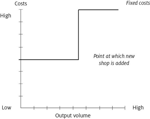
. This shows a static level of fixed costs over a particular range of output. To return to a previous example, this could show the fixed cost, rent and rates for a shop to be constant over a wide range of sales levels. Once the shop owner has reached a satisfactory sales and profit level in one shop, he or she may decide to rent another one, in which case the fixed costs will âstep' up. This can be shown in the variation on the fixed cost model in
Figure 1.2
.
FIGURE 1.1
 Â
Cost model
1
: showing fixed costs
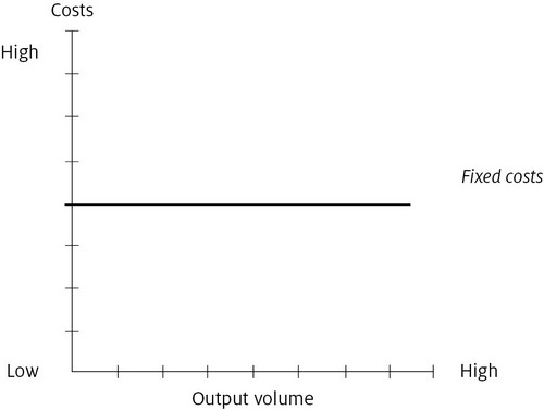
FIGURE 1.2
 Â
Variation on cost model
1
: showing a step up in fixed costs
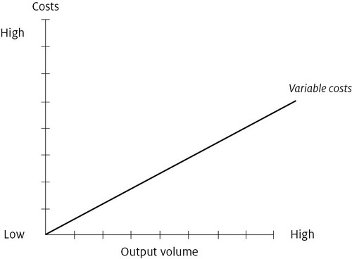
Variable costs
These are costs that change in line with output. Raw materials for production, packaging materials, bonuses, piece rates, sales commission and postage are some examples. The important characteristic of a variable cost is that it rises or falls in direct proportion to any growth or decline in output volumes. We can now draw a chart showing how variable costs behave as volume changes. The second phase of our cost model will look like
Figure 1.3
. There is a popular misconception that defines fixed costs as those costs that are predictable, and variable costs as those that are subject to change at any moment. The definitions already given are the only valid ones for costing purposes.
FIGURE 1.3
 Â
Cost model
2
: showing behaviour of variable costs as volume changes
Semi-variable costs
Unfortunately not all costs fit easily into either the fixed or variable category. Some costs have both a fixed and a variable element. For example, a mobile phone has a monthly rental cost which is fixed, and a cost per unit consumed over and above a set usage rate which is variable. In this particular example low consumers can be seriously penalized. If only a few calls are made each month, their total cost per call (fixed rental + cost per unit ÷ number of calls) can be several pounds.
Other examples of this dual-component cost are photocopier rentals, electricity and gas.
These semi-variable costs must be split into their fixed and variable elements. For most small businesses this will be a fairly simple process, nevertheless it is essential to do it accurately or else much of the purpose and benefits of this method of cost analysis will be wasted.
Bringing both fixed and variable costs together we can build a costing model that shows how total costs behave for different levels of output (
Figure 1.4
).
FIGURE 1.4
 Â
Cost model showing total costs and fixed costs
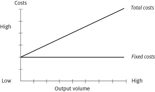
So any company capturing a sizeable market share will have an implied cost advantage over any competitor with a smaller market share. That cost advantage can then be used to make more profit, lower prices and compete for an even greater share of the market or invest in making the product better and so stealing a march on competitors. By starting the variable costs from the plateau of the fixed costs, we can produce a line showing the total costs. Taking vertical and horizontal lines from any point in the total cost line will give the total costs for any chosen output volume. This is an essential feature of the costing model that lets us see how costs change with different output volumes: in other words, accommodating the dynamic nature of a business. It is to be hoped that we are not simply producing things and creating costs. We are also selling things and creating income. So a further line can be added to the model to show sales revenue as it comes in. To help bring the model to life, let's add some figures, for illustration purposes only.