Data Mining (84 page)
Authors: Mehmed Kantardzic

In some applications, the transaction database has to be mined frequently to capture customer behavior. In such applications, the efficiency of data mining could be a more important factor than the complete accuracy of the results. In addition, in some applications the problem domain may be vaguely defined. Missing some marginal cases that have confidence and support levels at the borderline may have little effect on the quality of the solution to the original problem. Allowing imprecise results can in fact significantly improve the efficiency of the applied mining algorithm.
As the database size increases,
sampling
appears to be an attractive approach to data mining. A sampling-based algorithm typically requires two scans of the database. The algorithm first takes a sample from the database and generates a set of candidate itemsets that are highly likely to be frequent in the complete database. In a subsequent scan over the database, the algorithm counts these itemsets’ exact support and the support of their negative border. If no itemset in the negative border is frequent, then the algorithm has discovered all frequent itemsets. Otherwise, some superset of an itemset in the negative border could be frequent, but its support has not yet been counted. The sampling algorithm generates and counts all such potentially frequent itemsets in subsequent database scans.
Because it is costly to find frequent itemsets in large databases,
incremental updating
techniques should be developed to maintain the discovered frequent itemsets (and corresponding association rules) so as to avoid mining the whole updated database again. Updates on the database may not only invalidate some existing frequent itemsets but also turn some new itemsets into frequent ones. Therefore, the problem of maintaining previously discovered frequent itemsets in large and dynamic databases is nontrivial. The idea is to reuse the information of the old frequent itemsets and to integrate the support information of the new frequent itemsets in order to substantially reduce the pool of candidates to be reexamined.
In many applications, interesting associations among data items often occur at a relatively high
concept level
. For example, one possible hierarchy of food components is presented in Figure
10.5
, where M (milk) and B (bread), as concepts in the hierarchy, may have several elementary sub-concepts. The lowest level elements in the hierarchy (M
1
, M
2
, … , B
1
, B
2
, …) are types of milk and bread defined with their bar-codes in the store. The purchase patterns in a transaction database may not show any substantial regularities at the elementary data level, such as at the bar-code level (M
1
, M
2
, M
3
, B
1
, B
2
, … ), but may show some interesting regularities at some high concept level(s), such as milk M and bread B.
Figure 10.5.
An example of concept hierarchy for mining multiple-level frequent itemsets.
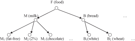
Consider the class hierarchy in Figure
10.5
. It could be difficult to find high support for purchase patterns at the primitive-concept level, such as chocolate milk and wheat bread. However, it would be easy to find in many databases that more than 80% of customers who purchase milk may also purchase bread. Therefore, it is important to mine frequent itemsets at a generalized abstraction level or at multiple-concept levels; these requirements are supported by the
Apriori
generalized-data structure.
One extension of the
Apriori
algorithm considers an
is-a
hierarchy on database items, where information about multiple abstraction levels already exists in the database organization. An
is-a
hierarchy defines which items are a specialization or generalization of other items. The extended problem is to compute frequent itemsets that include items from different hierarchy levels. The presence of a hierarchy modifies the notation of when an item is contained in a transaction. In addition to the items listed explicitly, the transaction contains their ancestors in the taxonomy. This allows the detection of relationships involving higher hierarchy levels, since an itemset’s support can increase if an item is replaced by one of its ancestors.
10.5 FP GROWTH METHOD
Let us define one of the most important problems with scalability of the
Apriori
algorithm. To generate one FP of length 100, such as {a
1
, a
2
, … , a
100
}, the number of candidates that has to be generated will be at least
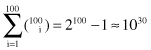
and it will require hundreds of database scans. The complexity of the computation increases exponentially. That is only one of the many factors that influence the development of several new algorithms for association-rule mining.
FP growth method
is an efficient way of mining frequent itemsets in large databases. The algorithm mines frequent itemsets without the time-consuming candidate-generation process that is essential for
Apriori
. When the database is large, FP growth first performs a database projection of the frequent items; it then switches to mining the main memory by constructing a compact data structure called the FP tree. For an explanation of the algorithm, we will use the transactional database in Table
10.2
and the minimum support threshold of 3.
TABLE 10.2.
The Transactional Database T
| TID | Itemset |
| 01 | f, a, c, d, g, i, m, p |
| 02 | a, b, c, f, l, m, o |
| 03 | b, f, h, j, o |
| 04 | b, c, k, s, p |
| 05 | a, f, c, e, l, p, m, n |
First, a scan of the database T derives a list L of frequent items occurring three or more than three times in the database. These are the items (with their supports):

The items are listed in descending order of frequency. This ordering is important since each path of the FP tree will follow this order.
Second, the root of the tree, labeled ROOT, is created. The database T is scanned a second time. The scan of the first transaction leads to the construction of the first branch of the FP tree: {(f,1), (c,1), (a,1), (m,1), (p,1)}. Only those items that are in the list of frequent items L are selected. The indices for nodes in the branch (all are 1) represent the cumulative number of samples at this node in the tree, and of course, after the first sample, all are 1. The order of the nodes is not as in the sample but as in the list of frequent items L. For the second transaction, because it shares items f, c, and a it shares the prefix {f, c, a} with the previous branch and extends to the new branch {(f, 2), (c, 2), (a, 2), (m, 1), (p, 1)}, increasing the indices for the common prefix by one. The new intermediate version of the FP tree, after two samples from the database, is given in Figure
10.6
a. The remaining transactions can be inserted similarly, and the final FP tree is given in Figure
10.6
b.
Figure 10.6.
FP tree for the database T in Table
10.2
. (a) FP tree after two samples; (b) final FT tree.
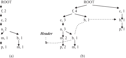
To facilitate tree traversal, an
item header table
is built, in which each item in list L connects nodes in the FP tree with its values through node links. All f nodes are connected in one list, all c nodes in the other, and so on. For simplicity of representation only the list for b nodes is given in Figure
10.6
b. Using the compact-tree structure, the FP growth algorithm mines the complete set of frequent itemsets.
According to the list L of frequent items, the complete set of frequent itemsets can be divided into subsets (six for our example) without overlap: (1) frequent itemsets having item p (the end of list L); (2) the itemsets having item m but not p; (3) the frequent itemsets with b and without both m and p; … ; and (6) the large itemsets only with f. This classification is valid for our example, but the same principles can be applied to other databases and other L lists.
Based on node-link connection, we collect all the transactions that p participates in by starting from the header table of p and following p’s node links. In our example, two paths will be selected in the FP tree: {(f,4), (c,3), (a,3), (m,2), (p,2)} and {(c,1), (b,1), (p,1)}, where samples with a frequent item p are {(f,2), (c,2), (a,2), (m,2), (p,2)}, and {(c,1), (b,1), (p,1)}. The given threshold value (3) satisfies only the frequent itemsets
{(c,3), (p,3)},
or the simplified
{c, p}
. All other itemsets with p are below the threshold value.
The next subsets of frequent itemsets are those with m and without p. The FP tree recognizes the paths {(f,4), (c,3), (a,3), (m,2)}, and {(f,4), (c,3), (a,3), (b,1), (m,1)}, or the corresponding accumulated samples {(f,2), (c,2), (a,2), (m,2)}, and {(f,1), (c,1), (a,1), (b,1), (m,1)}. Analyzing the samples we discover the frequent itemset
{(f,3), (c,3), (a,3), (m,3)}
or, simplified,
{f, c, a, m}
.
Repeating the same process for subsets (3) to (6) in our example, additional frequent itemsets could be mined. These are itemsets
{f, c, a}
and
{f, c}
, but they are already subsets of the frequent itemset
{f, c, a, m}
. Therefore, the final solution in the FP growth method is the set of frequent itemsets, which is, in our example,
{{c, p}, {f, c, a, m}}.
Experiments have shown that the FP growth algorithm is faster than the
Apriori
algorithm by about one order of magnitude. Several optimization techniques are added to the FP growth algorithm, and there exists its versions for mining sequences and patterns under constraints.
10.6 ASSOCIATIVE-CLASSIFICATION METHOD
CMAR is a classification method adopted from the FP growth method for generation of frequent itemsets. The main reason we included CMAR methodology in this chapter is its FP growth roots, but there is the possibility of comparing CMAR accuracy and efficiency with the C4.5 methodology.