Data Mining (82 page)
Authors: Mehmed Kantardzic

Miyamoto, S.,
Fuzzy Sets in Information Retrieval and Cluster Analysis
, Cluver Academic Publishers, Dodrecht, Germany, 1990.
This book offers an in-depth presentation and analysis of some clustering algorithms and reviews the possibilities of combining these techniques with fuzzy representation of data. Information retrieval, which, with the development of advanced Web-mining techniques, is becoming more important in the data-mining community, is also explained in the book.
10
ASSOCIATION RULES
Chapter Objectives
- Explain the local modeling character of association-rule techniques.
- Analyze the basic characteristics of large transactional databases.
- Describe the Apriori algorithm and explain all its phases through illustrative examples.
- Compare the frequent pattern (FP) growth method with the Apriori algorithm.
- Outline the solution for association-rule generation from frequent itemsets.
- Explain the discovery of multidimensional associations.
- Introduce the extension of FP growth methodology for classification problems.
When we talk about machine-learning methods applied to data mining, we classify them as either parametric or nonparametric methods. In
parametric methods
used for density estimation, classification, or regression, we assume that a final model is valid over the entire input space. In regression, for example, when we derive a linear model, we apply it for all future inputs. In classification, we assume that all samples (training, but also new, testing) are drawn from the same density distribution. Models in these cases are global models valid for the entire n-dimensional space of samples. The advantage of a parametric method is that it reduces the problem of modeling with only a small number of parameters. Its main disadvantage is that initial assumptions do not hold in many real-world problems, which causes a large error. In
nonparametric estimation
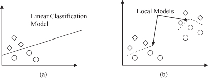
, all we assume is that similar inputs have similar outputs. Methods do not assume any a priori density or parametric form. There is no single global model. Local models are estimated as they occur, affected only by nearby training samples (Fig.
10.1
).
Figure 10.1.
Parametric versus nonparametric methods. (a) Parametric methods build global models; (b) nonparametric methods result in local modelling.
The discovery of association rules is one of the major techniques of data mining, and it is perhaps the most common form of local-pattern discovery in unsupervised learning systems. It is a form of data mining that most closely resembles the process that most people think about when they try to understand the data-mining process, namely, “mining” for gold through a vast database. The gold in this case would be a rule that is interesting, that tells you something about your database that you did not already know and probably were not able to explicitly articulate. These methodologies retrieve all possible interesting patterns in the database. This is a strength in the sense that it leaves “no stone unturned.” But it can be viewed also as a weakness because the user can easily become overwhelmed with a large amount of new information, and an analysis of their usability is difficult and time-consuming.
Besides the standard methodologies such as the Apriori technique for association-rule mining, we will explain some extensions such as
FP tree
and Classification Based on Multiple Association Rules (CMAR) algorithms. All these methodologies show how important and applicable the problem of market-basket analysis is and the corresponding methodologies for discovery of association rules in data.
10.1 MARKET-BASKET ANALYSIS
A market basket is a collection of items purchased by a customer in a single transaction, which is a well-defined business activity. For example, a customer’s visits to a grocery store or an online purchase from a virtual store on the Web are typical customer transactions. Retailers accumulate huge collections of transactions by recording business activities over time. One common analysis run against a transactions database is to find sets of items, or
itemsets
, that appear together in many transactions. A business can use knowledge of these patterns to improve the placement of these items in the store or the layout of mail-order catalog pages and Web pages. An itemset containing
i
items is called an
i-itemset
. The percentage of transactions that contain an itemset is called the itemset’s
support
. For an itemset to be interesting, its support must be higher than a user-specified minimum. Such itemsets are said to be frequent.
Why is finding frequent itemsets a nontrivial problem? First, the number of customer transactions can be very large and usually will not fit in a central memory of a computer. Second, the potential number of frequent itemsets is exponential to the number of different items, although the actual number of frequent itemsets can be much smaller. Therefore, we want algorithms that are scalable (their complexity should increase linearly, not exponentially, with the number of transactions) and that examine as few infrequent itemsets as possible. Before we explain some of the more efficient algorithms, let us try to describe the problem more formally and develop its mathematical model.
From a database of sales transactions, we want to discover the important associations among items such that the presence of some items in a transaction will imply the presence of other items in the same transaction. Let I = {i
1
, i
2
, … , i
m
} be a set of literals, called items. Let DB be a set of transactions, where each transaction T is a set of items such that T ⊆ I. Note that the quantities of the items bought in a transaction are not considered, meaning that each item is a binary variable indicating whether an item was bought or not. Each transaction is associated with an identifier called a transaction identifier or TID. An example of the model for such a transaction database is given in Table
10.1
.
TABLE 10.1.
A Model of A Simple Transaction Database
| Database DB: | |
| TID | Items |
| 001 | A C D |
| 002 | B C E |
| 003 | A B C E |
| 004 | B E |
Let X be a set of items. A transaction T is said to contain X if and only if X ⊆ T. An association rule implies the form X ⇒ Y, where X ⊆ I, Y ⊆ I, and X ∩Y = Ø. The rule X ⇒ Y holds in the transaction set DB with
confidence c
if
c
% of the transactions in DB that contain X also contain Y. The rule X ⇒ Y has
support s
in the transaction set DB if
s
% of the transactions in DB contain X ∪ Y. Confidence denotes the strength of implication and support indicates the frequency of the patterns occurring in the rule. It is often desirable to pay attention to only those rules that may have a reasonably large support. Such rules with high confidence and strong support are referred to as
strong rules
. The task of mining association rules is essentially to discover strong association rules in large databases. The problem of mining association rules may be decomposed into two phases:
1.
Discover the large itemsets, that is, the sets of items that have transaction support
s
above a predetermined minimum threshold.
2.
Use the large itemsets to generate the association rules for the database that have confidence
c
above a predetermined minimum threshold.
The overall performance of mining association rules is determined primarily by the first step. After the large itemsets are identified, the corresponding association rules can be derived in a straightforward manner. Efficient counting of large itemsets is thus the focus of most mining algorithms, and many efficient solutions have been designed to address previous criteria. The
Apriori
algorithm provided one early solution to the problem, and it will be explained in greater detail in this chapter. Other subsequent algorithms built upon the
Apriori
algorithm represent refinements of a basic solution and they are explained in a wide spectrum of articles including texts recommended in Section 10.10.
10.2 ALGORITHM
APRIORI
The algorithm
Apriori
computes the frequent itemsets in the database through several iterations. Iteration
i
computes all frequent
i
-itemsets (itemsets with
i
elements). Each iteration has two steps:
candidate generation
and
candidate counting and selection
.
In the first phase of the first iteration, the generated set of candidate itemsets contains all 1-itemsets (i.e., all items in the database). In the counting phase, the algorithm counts their support by searching again through the whole database. Finally, only 1-itemsets (items) with s above required threshold will be selected as frequent. Thus, after the first iteration, all frequent 1-itemsets will be known.
What are the itemsets generated in the second iteration? In other words, how does one generate 2-itemset candidates? Basically, all pairs of items are candidates. Based on knowledge about infrequent itemsets obtained from previous iterations, the
Apriori
algorithm reduces the set of candidate itemsets by pruning—
a priori
—those candidate itemsets that cannot be frequent. The pruning is based on the observation that if an itemset is frequent all its subsets could be frequent as well. Therefore, before entering the candidate-counting step, the algorithm discards every candidate itemset that has an infrequent subset.
Consider the database in Table
10.1
. Assume that the minimum support s = 50%, so an itemset is frequent if it is contained in at least 50% of the transactions—in our example, in two out of every four transactions in the database. In each iteration, the
Apriori
algorithm constructs a candidate set of large itemsets, counts the number of occurrences of each candidate, and then determines large itemsets based on the predetermined minimum support s = 50%.
In the first step of the first iteration, all single items are candidates.
Apriori
simply scans all the transactions in a database DB and generates a list of candidates. In the next step, the algorithm counts the occurrences of each candidate and based on threshold s selects frequent itemsets. All these steps are given in Figure
10.2
. Five 1-itemsets are generated in C
1
and, of these, only four are selected as large in L
1
because their support is greater than or equal to two, or s ≥ 50%.
Figure 10.2.
First iteration of the
Apriori
algorithm for a database DB. (a) Generate phase; (b1) count phase; (b2) select phase.

To discover the set of large 2-itemsets, because any subset of a large itemset could also have minimum support, the
Apriori
algorithm uses L
1
*L
1
to generate the candidates. The operation * is defined in general as

For k = 1 the operation represents a simple concatenation. Therefore, C
2
consists of 2-itemsets generated by the operation|L
1
· (|L
1
|−1)/2 as candidates in the second iteration. In our example, this number is 4 · 3/2 = 6. Scanning the database DB with this list, the algorithm counts the support for every candidate and in the end selects a large 2-itemsets L
2
for which s ≥ 50%. All these steps and the corresponding results of the second iteration are given in Figure
10.3
.