Data Mining (83 page)
Authors: Mehmed Kantardzic

Figure 10.3.
Second iteration of the
Apriori
algorithm for a database DB. (a) Generate phase; (b1) count phase; (b2) select phase
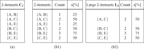
The set of candidate itemset C
3
is generated from L
2
using the previously defined operation L
2
*L
2
. Practically, from L
2
, two large 2-itemsets with the same first item, such as {B, C} and {B, E}, are identified first. Then,
Apriori
tests whether the 2-itemset {C, E}, which consists of the second items in the sets {B, C} and {B, E}, constitutes a large 2-itemset or not. Because {C, E} is a large itemset by itself, we know that all the subsets of {B, C, E} are large, and then {B, C, E} becomes a candidate 3-itemset. There is no other candidate 3-itemset from L
2
in our database DB.
Apriori
then scans all the transactions and discovers the large 3-itemsets L
3
, as shown in Figure
10.4
.
Figure 10.4.
Third iteration of the
Apriori
algorithm for a database DB. (a) Generate phase; (b1) count phase; (b2) select phase

In our example, because there is no candidate 4-itemset to be constituted from L
3
,
Apriori
ends the iterative process.
Apriori
counts not only the support of all frequent itemsets, but also the support of those infrequent candidate itemsets that could not be eliminated during the pruning phase. The set of all candidate itemsets that are infrequent but whose support is counted by
Apriori
is called the
negative border
. Thus, an itemset is in the negative border if it is infrequent, but all its subsets are frequent. In our example, analyzing Figures
10.2
and
10.3
, we can see that the negative border consists of itemsets {D}, {A, B}, and {A, E}. The negative border is especially important for some improvements in the
Apriori
algorithm such as increased efficiency in the generation of large itemsets.
10.3 FROM FREQUENT ITEMSETS TO ASSOCIATION RULES
The second phase in discovering association rules based on all frequent i-itemsets, which have been found in the first phase using the
Apriori
or some other similar algorithm, is relatively simple and straightforward. For a rule that implies {x
1
,x
2
, x
3
} → x
4
, it is necessary that both itemset {x
1
, x
2
, x
3
, x
4
} and {x
1
, x
2
, x
3
} are frequent. Then, the confidence
c
of the rule is computed as the quotient of supports for the itemsets
c
=
s
(x
1
,x
2
,x
3
,x
4
)/
s
(x
1
,x
2
,x
3
). Strong association rules are rules with a confidence value
c
above a given threshold.
For our example of database DB in Table
10.1
, if we want to check whether the association rule {B, C} → E is a strong rule, first we select the corresponding supports from tables L
2
and L
3
:
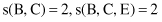
and using these supports we compute the confidence of the rule:

Whatever the selected threshold for strong association rules is (e.g., c
T
= 0.8 or 80%), this rule will pass because its confidence is maximal, that is, if a transaction contains items B and C, it will also contain item E. Other rules are also possible for our database DB, such as A → C because c(A → C) = s(A, C)/s(A) = 1, and both itemsets {A} and {A, C} are frequent based on the
Apriori
algorithm. Therefore, in this phase, it is necessary only to systematically analyze all possible association rules that could be generated from the frequent itemsets, and select as strong association rules those that have a confidence value above a given threshold.
Notice that not all the discovered strong association rules (i.e., passing the required support
s
and required confidence
c
) are interesting enough to be presented and used. For example, consider the following case of mining the survey results in a school of 5000 students. A retailer of breakfast cereal surveys the activities that the students engage in every morning. The data show that 60% of the students (i.e., 3000 students) play basketball; 75% of the students (i.e., 3750 students) eat cereal; and 40% of them (i.e., 2000 students) play basketball and also eat cereal. Suppose that a data-mining program for discovering association rules is run on the following settings: the minimal support is 2000 (s = 0.4) and the minimal confidence is 60% (c = 0.6). The following association rule will be produced: “(play basketball) → (eat cereal),” since this rule contains the minimal student support and the corresponding confidence c = 2000/3000 = 0.66 is larger than the threshold value. However, the above association rule is misleading since the overall percentage of students eating cereal is 75%, larger than 66%. That is, playing basketball and eating cereal are in fact negatively associated. Being involved in one itemset decreases the likelihood of being involved in the other. Without fully understanding this aspect, one could make wrong business or scientific decisions from the association rules derived.
To filter out such misleading associations, one may define that an association rule A → B is
interesting
if its confidence exceeds a certain measure. The simple argument we used in the example above suggests that the right heuristic to measure association should be
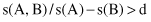
or alternatively:
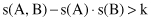
where d or k are suitable constants. The expressions above essentially represent tests of statistical independence. Clearly, the factor of statistical dependence among analyzed itemsets has to be taken into consideration to determine the usefulness of association rules. In our simple example with students this test fails for the discovered association rule

and, therefore, despite high values for parameters s and c, the rule is not interesting. In this case, it is even misleading.
10.4 IMPROVING THE EFFICIENCY OF THE
APRIORI
ALGORITHM
Since the amount of the processed data in mining frequent itemsets tends to be huge, it is important to devise efficient algorithms to mine such data. Our basic
Apriori
algorithm scans the database several times, depending on the size of the largest frequent itemset. Since Apriori algorithm was first introduced and as experience has accumulated, there have been many attempts to devise more efficient algorithms of frequent itemset mining including approaches such as hash-based technique, partitioning, sampling, and using vertical data format. Several refinements have been proposed that focus on reducing the number of database scans, the number of candidate itemsets counted in each scan, or both.
Partition
-
based Apriori
is an algorithm that requires only two scans of the transaction database. The database is divided into disjoint partitions, each small enough to fit into available memory. In a first scan, the algorithm reads each partition and computes locally frequent itemsets on each partition. In the second scan, the algorithm counts the support of all locally frequent itemsets toward the complete database. If an itemset is frequent with respect to the complete database, it must be frequent in at least one partition. That is the heuristics used in the algorithm. Therefore, the second scan through the database counts itemset’s frequency only for a union of all locally frequent itemsets. This second scan directly determines all frequent itemsets in the database as a subset of a previously defined union.