The Numbers Behind NUMB3RS (20 page)
Read The Numbers Behind NUMB3RS Online
Authors: Keith Devlin

But direct connections are not all that matters. Another important notion is the “distance” between two nodes. Any two nodes are considered connected (possibly indirectly) if there is some path between themâthat is, some sequence of nodes starting at one and ending at the other, with each node connected to the next by an edge. In other words, a path is a route between two nodes where one travels along edges, using intermediate nodes as “stepping-stones.” The length of a path is the number of edges it contains, and the shortest possible length of a path between nodes A and B is called the distance between them, denoted by d(A,B). Paths that have this shortest possible length are called geodesic paths. In particular, every edge is a geodesic path of length 1.
The notion of distance between nodes leads to other ways of identifying key nodesâthat is, it leads to other measures of centrality that can be used to give each node a “score” that reflects something about its potential importance. The concept of “betweenness” gives each node a score that reflects its role as a stepping-stone along geodesic paths between other pairs of nodes. The idea is that if a geodesic path from A to B (there may be more than one) goes through C, then C gains potential importance. More specifically, the betweenness of C as a link between A and B is defined as
Â
the number of geodesic paths from A to B that go through C
Â
divided by
Â
the number of geodesic paths from A to B.
Â
The overall betweenness score of C is calculated by adding up the results of these calculations for all possible examples of A and B. Here is an example of a node in a graph having low degree but high betweenness:

Such nodesâor the people they represent in a human networkâcan have important roles in providing connections between sets of nodes that otherwise have few other connections, or perhaps no other connections.
The third “centrality measure” used by Krebs, and shown in the table above, is the “closeness” score. Roughly speaking, it indicates for each node how close it is to the other nodes in the graph. For a node C, you first calculate the distances d(C,A), d(C,B), and so on, to all of the other nodes in the graph. Then you add the reciprocals of these distancesâthat is, you calculate the sum

The smaller the distances are between C and other nodes, the larger these reciprocals will be. For example, if C has 10 nodes at distance 1 (so C has degree 10), then the closeness calculation starts with 10 ones, and if there are an additional 60 nodes at distance 2, then we add “
1
/2” 60 times, and if there are 240 nodes at distance 3, then we add “
1
/3” 540 times, getting

Whereas degree measures count only immediately adjacent nodes, closeness gives credit for having many nodes at distance 2, many more at distance 3, and so on. Analysts consider closeness a good indication of how rapidly information can spread through a network from one node to others.
RANDOM GRAPHS: USEFUL TOOLS IN UNDERSTANDING LARGE NETWORKS
The amount of detailed information contained in a large graph, such as the graphs generated by the NSA in monitoring communications including phone calls or computer messages in regions such as the Middle East, is so huge that mathematicians naturally want to find “scaled-down models” for themâsimilar graphs that are small enough that their features can be studied and understood, and which can then provide clues about what to look for in analyzing the actual graphs. Recent research on graphs and networks has led to an explosion of interest in what are called random graphs. These graphs can help not only in understanding the structural features of large graphs and networks, but in estimating how much information is missing in a graph constructed from incomplete data. Since it is virtually impossible to get complete data about communications and relationships between people in a networkâparticularly a covert networkâthis kind of estimation is critically important.
Interest in the study of random graphs was sparked in the late 1950s by the research of two Hungarian mathematicians, Paul Erdös and Alfred Renyi. What they investigated were quite simple models of random graphs. The most important one works like this:
Take a certain number of nodes n. Consider every pair of nodes (there are n à (nâ1)/2 pairs) and decide for each of these pairs whether they are connected by an edge by a random experimentânamely, flip a coin that has probability p of coming up heads, and insert an edge whenever the flip results in heads.
Thus, every edge occurs at random, and its occurrence (or not) is entirely unaffected by the presence or absence of other edges. Given its random construction you might think that there is little to say about such a graph, but the opposite turns out to be the case. Studying random graphs has proved useful, particularly in helping mathematicians understand the important structural idea called graph components. If every node in a graph has a path leading to every other node, the graph is said to be connected. Otherwise, the nodes of the graph can be separated into two or more componentsâsets of nodes within which any two are connected by some path, but with no paths connecting nodes belonging to different components. (This is a mathematician's way of describing the “You can't get there from here” phenomenon.)
Erdös and Renyi showed that values of p close to 1/n are critical in determining the size and number of components in a random graph. (Note that any one node will be connected by an edge to (nâ1) à p other nodesâon average. So if p is close to 1/n the average degree of all the nodes is about 1.) Specifically, Erdös and Renyi demonstrated that if the number of edges is smaller than the number of nodes by some percentage, then the graph will tend to be sparsely connectedâwith a very large number of componentsâwhereas if the number of edges is larger by some percentage than the number of nodes, the graph will likely contain one giant component that contains a noticeable fraction of the nodes, but the second-largest component will likely be much smaller. Refinements of these results are still a subject of interesting mathematical research.
The study of random graphs has seen an explosion of interest in the late 1990s and early 2000s on the part of both pure mathematicians and social network analysts, largely thanks to the realization that there are far more flexible and realistic probability models for the sorts of graphs seen in real-world networks.
Since real-world networks are constantly evolving and changing, the mathematical investigation of random graphs has focused on models that describe the growth of graphs. In a very influential paper written in 1999, Albert Barabasi and Reka Albert proposed a model of preferential attachment, in which new nodes are added to a graph and have a fixed quota of edges, which are randomly connected to previously existing nodes with probabilities proportional to the degrees of the existing nodes. This model achieved stunning success in describing a very important graphânamely, the graph whose nodes are websites and whose connections are links between websites. It also succeeded in providing a mechanism for generating graphs in which the frequency of nodes of different degrees follows a
power law distribution
âthat is, the proportion of nodes that have degree
n
is roughly proportional to
1
/
n
3
. Later research has yielded methods of “growing” random graphs that have arbitrary powers like
n
2.4
or
n
2.7
in place of
n
3
. Such methods can be useful in modeling real-world networks.
SIX DEGREES OF SEPARATION: THE “SMALL WORLD” PHENOMENON
Another line of mathematical research that has recently attracted the attention of network analysts is referred to as the “small world model.” The catalyst was a 1998 paper by Duncan Watts and Steven Strogatz, in which they showed that within a large network the introduction of a few random long-distance connections tends to dramatically reduce the diameter of the networkâthat is, greatest distance between nodes in the network. These “transitory shortcuts” are often present in real-world networksâin fact, Krebs' analysis of the 9/11 terrorist network described judiciously timed meetings involving representatives of distant branches of the Al Qaeda network to coordinate tasks and report progress in preparing for those attacks.
The most famous study of such a phenomenon was published by social psychologist Stanley Milgram in 1967, who suggested that if two U.S. citizens were picked at random they would turn out to be connected on average by a chain of acquaintances of length six. Milgram's basis for that claim was an experiment, in which he recruited sixty people in Omaha, Nebraska, to forward (by hand!) letters to a particular stockbroker in Massachusetts by locating intermediaries who might prove to be “a friend of a friend of a friend.” In fact only three of fifty attempts reached the target, but the novelty and appeal of the experiment and the concept underlying it ensured its lasting fame.
The more substantial work of Watts and Strogatz has led to more accurate and useful research, but the “six degrees” idea has gained such a strong foothold that mythology dominates fact in popular thinking about the subject. The phrase “six degrees of separation” originated in the title of a 1991 play by John Guare, in which a woman tells her daughter, “â¦everybody on the planet is separated by only six other peopleâ¦. I am bound, you are bound, to everyone on this planet by a trail of six people. It is a profound thought.” It's not true, but it's an intriguing idea.
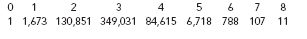
What does in fact seem to be true is that the diameters of networksâthe longest path lengths (or average path lengths) between nodesâare smaller than one would expect based on the sheer size of the networks. There are two intriguing examples that are much talked about in widely separated fields. In the movie business, the “Kevin Bacon game” concerns the connections between film actors. Using actors as nodes of a graph, consider two actors as connected by an edge if they have appeared in at least one movie together. Because the actor Kevin Bacon has appeared in movies with a great many other actors, the idea originated some years ago to show that two actors are not far apart in this graph if both have a small “Bacon number,” defined as their geodesic distance from Kevin Bacon. Thus, an actor who appeared in a movie with Kevin would have a Bacon number of 1, and an actor who never appeared with him but was in a movie with someone whose Bacon Number is 1 would have a Bacon number of 2, and so on. A recent study yielded the following distribution of Bacon numbers: