The 30 Day MBA (16 page)
Authors: Colin Barrow

With this method, dividends are assumed to grow in the future at the constant rate achieved by averaging the last few years' performance.
Capital asset pricing model (CAPM)
Before turning to the next method, we need to clarify some aspects of risk. There are two broad types of risk:
- Specific risk: This applies to one particular business. It includes, for example, the risk of losing the chief executive; the risk of someone else bringing out a similar or better product; or the risk of labour problems. Shareholders are expected not to want compensation for this type of risk as it can be diversified away by holding a sufficient number of investments in their portfolios.
- Systematic risk: This derives from global or macroeconomic events that can damage all investments to some extent and therefore holders require compensation for this risk to their wealth. This compensation takes the form of a higher required rate of return.
A slightly more complicated approach to the cost of equity tries to take the systematic risk element into account. It is known as the capital asset pricing model or CAPM for short. Put simply, CAPM states that investors' required rate of return on a share is composed of two parts: a risk-free rate similar to that obtainable on a risk-free investment in short-term government securities; and an additional premium to compensate for the systematic risk involved in investing in shares.
This systematic risk for a company's shares is measured by the size of its beta factor. A beta the size of 1.0 for a company means that its shares have the same systematic risk as the average for the whole market. If the beta is 1.4 then systematic risk for the share is 40 per cent higher than the market average. A company's share beta is applied to the market premium that is obtained from the excess of the return on a market portfolio of shares over the risk-free rate of return. The formula to calculate cost of equity capital using CAPM is:
Ke = Rf + B(Rm â Rf)
Where: Ke = cost of equity, Rf = risk-free return, Rm = return on market portfolio of shares and B = beta factor.
Example
If the risk-free rate of return is 5.5 per cent and the return on a market portfolio is 12 per cent, then for a company with a beta of 0.7 for its ordinary shares calculate its cost of equity.

Of the two methods described for finding the cost of equity for a company, the latter CAPM method is the more scientific. Ideally, the risk-free and market rates of return should reflect the future, but current rates of return are used as substitutes. Beta factors measure how sensitive each company's
share price movements are relative to market movements over a period of a few years.
The weakness of CAPM is that it assumes all investors are rational and well informed, that markets are perfect and that there is an unlimited supply of risk-free money. There are even more complex models for calculating the cost of equity capital, but none are without their critics.
Weighted average cost of capital
Having identified the cost of equity and the cost of borrowed capital (and that of any other long-term source of finance such as hire purchase or mortgages), we need to combine them into one overall cost of capital. This is primarily for use in project appraisals as justification of those that yield a return in excess of their cost of capital.
An average cost is required because we do not usually identify each individual project with one particular source of finance. Because equity and debt capital have very different costs, we would make illogical decisions and accept a project financed by debt capital only to reject a similar project next time round when it was financed by equity capital. Generally businesses take the view that all projects have been financed from a common pool of money except for the relatively rare case when project-specific finance is raised. The weightings used in the calculations should be based on the market value of the securities and not on their book or balance sheet values.
Example
Assume your company intends to keep the gearing ratio of borrowed capital to equity in the proportion of 20 : 80. The nominal cost of new capital from these sources has been assessed, say, at 10 per cent and 15 per cent respectively and corporation tax is 30 per cent. The calculation of the overall weighted average cost is as follows:
Type of capital | Proportion (a) | After-tax cost (b) | Weighted cost (a à b) |
10% loan capital | 0.20 | 7.0% | 1.4% |
Equity | 0.80 | 15.0% | 12.0% |
13.4% |
The resulting weighted average cost of 13.4 per cent is the minimum rate that this company should accept on proposed investments. Any investment that is not expected to achieve this return is not a viable proposition. Risk has been allowed for in the calculation of the beta factor used in the CAPM method of identifying the cost of equity. This relates to the risk of the
existing whole business. If a company embarks on a project of significantly different risk, or has a divisional structure of activities of varying risk levels, then a single cost of equity for the whole company is inappropriate. In this situation, the average beta of proxy companies operating in the same field as a division can be used.
The cost of capital is an important figure as it is in essence the threshold for future investments. Taking the figures shown above, if our weighted average cost of capital is 13.4 per cent then taking on any new activity that makes a lower profit ratio will be lowering the performance, hardly an MBA type of activity.
Investment decisions, where the decisions have cost and revenue implications for years, perhaps even decades, fall into a number of categories:
- Bolt-on investments: These are where an investment will be supporting and enhancing an existing operation. For example, if part of a production process is being slowed down for want of some new equipment to eliminate a bottleneck.
- Standalone single project: This involves a simple accept or reject decision.
- Competing projects: This requires a choice of which produces the best results, either because only one can be pursued or because of limited finance. In the latter case this is described as capital rationing.
CASE STUDY
 Â
Cobra Beer
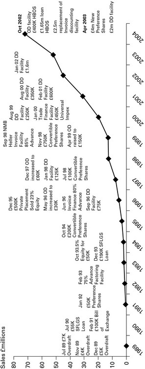
In 1990, Cambridge-educated and recently qualified accountant Karan Bilimoria started importing and distributing Cobra beer, a name he chose because it appeared to work well in lots of different languages. He initially supplied his beer to complement Indian restaurant food in the UK. Lord Bilimoria, as he now is, started out with debts of £20,000, but from a small flat in Fulham and with just a Citroen CV by way of assets he has grown his business to sales of over £100 million a year. Three factors have been key to its success. Cobra was originally sold in large 660ml bottles and so were more likely to be shared by diners. Also, as Cobra is less fizzy than European lagers, drinkers are less likely to feel bloated and can eat and drink more. The third factor was Bilimoria's extensive knowledge, through his training as an accountant, of sources of finance for a growing business. He was fortunate in having an old-style bank manager who had such belief in Cobra that he agreed a loan of £30,000, but since then he has had to tap into every possible type of funding (see
Figure 2.3
), including selling a 28 per cent stake in his firm in 1995.
FIGURE
2.3
 Â
Cobra Beer's financing strategy
What follows is an examination of the financial aspects of investment decisions. There may well be other strategic reasons for taking investment decisions, including those that might be more important than finance alone. For example, it could be imperative to deny a competitor a particular opportunity; or if part of achieving a national or global strategy calls for disproportionate expenses in one or more areas. However, there are NO circumstances when any investment decision should not be subjected to proper financial appraisal and so at least see the cost of accepting a lower return than required by the cost of capital being used.
Also, it's important to note that any methodology for appraising investments requires that cash is used rather than profits, for reasons that will become apparent as the techniques are explained. Profit is not ignored; it is simply allowed to work its way through in the timing of events.
Payback period
The most popular method for evaluating investment decisions is the payback method. To arrive at the payback period you have to work out how many years it takes to recover your cash investment.
Table 2.2
shows two investment projects that require respectively $/£/â¬20,000 and $/£/â¬40,000 cash now in order to get a series of cash returns spread over the next five years.
TABLE 2.2
 Â
The payback method
Investment A | Investment B | |
$/£/⬠| $/£/⬠| |
Initial cash cost NOW (Year 0) | 20,000 | 40,000 |
Net cash flows | ||
Year 1 | 1,000 | 10,000 |
Year 2 | 4,000 | 10,000 |
Year 3 | 8,000 | 16,000 |
Year 4 | 7,000 | 4,000 |
Year 5 | 5,000 | 28,000 |
Total cash in over period | 25,000 | 68,000 |
Cash surplus | 5,000 | 28,000 |
Although both propositions call for different amounts of cash to be invested, we can see that both recover all their cash outlays by year 4. So we can say these investments have a four-year payback. But as a matter of fact Investment B produces a much bigger surplus than the other project and it returns half our initial cash outlay in two years. Investment A has returned only a quarter of our cash over that time period.
Payback may be simple, but it is not much use when it comes to dealing with the timing or with comparing different investment amounts.
Discounted cash flow
We know intuitively that getting cash in sooner is better than getting it in later. In other words, a pound received now is worth more than a pound that will arrive in one, two or more years in the future because of what we could do with that money ourselves, or because of what we ourselves have to pay out to have use of that money (see Cost of capital above). To make sound investment decisions we need to ascribe a value to a future stream of earnings to arrive at what is known as the present value. If we know we could earn 20 per cent on any money we have, then the maximum we would be prepared to pay for a pound coming in one year hence would be around 80p. If we were to pay one pound now to get a pound back in a year's time we would in effect be losing money.
The technique used to handle this is known as discounting. The process is termed discounted cash flow (DCF) and the residual discounted cash is called the net present value.
The first column in
Table 2.3
shows the simple cash-flow implications of an investment proposition; a surplus of $/£/â¬5,000 comes after five years from putting $/£/â¬20,000 into a project. But if we accept the proposition that future cash is worth less than current cash, the only question we need to answer is how much less. If we take our weighted average cost of capital as a sensible starting point, we would select 13.4 per cent as an appropriate
rate at which to discount future cash flows. To keep the numbers simple and to add a small margin of safety, let's assume that 15 per cent is the rate we have selected (this doesn't matter too much, as you will see in the section on internal rate of return).