Data Mining (12 page)
Authors: Mehmed Kantardzic

If we select the threshold value for normal distribution of data as

then, all data that are out of range [−54.1, 131.2] will be potential outliers. Additional knowledge of the characteristics of the feature (age is always greater then 0) may further reduce the range to [0, 131.2]. In our example there are three values that are outliers based on the given criteria: 156, 139, and −67. With a high probability we can conclude that all three of them are typo errors (data entered with additional digits or an additional “–” sign).
An additional single-dimensional method is Grubbs’ method (Extreme Studentized Deviate), which calculates a Z value as the difference between the mean value for the attribute and the analyzed value divided by the standard deviation for the attribute. The Z value is compared with a 1% or 5% significance level showing an outlier if the Z parameter is above the threshold value.
In many cases multivariable observations cannot be detected as outliers when each variable is considered independently. Outlier detection is possible only when multivariate analysis is performed, and the interactions among different variables are compared within the class of data. An illustrative example is given in Figure
2.7
where separate analysis of each dimension will not give any outlier, but analysis of 2-D samples (x,y) gives one outlier detectable even through visual inspection.
Statistical methods for multivariate outlier detection often indicate those samples that are located relatively far from the center of the data distribution. Several distance measures can be implemented for such a task. The Mahalanobis distance measure includes the inter-attribute dependencies so the system can compare attribute combinations. It is a well-known approach that depends on estimated parameters of the multivariate distribution. Given
n
observations
x
i
from a p-dimensional data set (often
n p), denote the sample mean vector by
 n
n
and the sample covariance matrix by V
n
, where

The
Mahalanobis
distance for each multivariate data point
i (i
= 1, … ,
n
) is denoted by
M
i
and given by
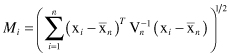
Accordingly, those n-dimensional samples with a large
Mahalanobis
distance are indicated as outliers. Many statistical methods require data-specific parameters representing a priori data knowledge. Such information is often not available or is expensive to compute. Also, most real-world data sets simply do not follow one specific distribution model.
Distance-based techniques
are simple to implement and make no prior assumptions about the data distribution model. However, they suffer exponential computational growth as they are founded on the calculation of the distances between all samples. The computational complexity is dependent on both the dimensionality of the data set m and the number of samples n and usually is expressed as O(n
2
m). Hence, it is not an adequate approach to use with very large data sets. Moreover, this definition can lead to problems when the data set has both dense and sparse regions. For example, as the dimensionality increases, the data points are spread through a larger volume and become less dense. This makes the convex hull harder to discern and is known as the “curse of dimensionality.”
Distance-based outlier detection method, presented in this section, eliminates some of the limitations imposed by the statistical approach. The most important difference is that this method is applicable to multidimensional samples while most of statistical descriptors analyze only a single dimension, or several dimensions, but separately. The basic computational complexity of this method is the evaluation of distance measures between all samples in an n-dimensional data set. Then, a sample s
i
in a data set S is an outlier if at least a fraction p of the samples in S lies at a distance greater than d. In other words, distance-based outliers are those samples that do not have enough neighbors, where neighbors are defined through the multidimensional distance between samples. Obviously, the criterion for outlier detection is based on two parameters, p and d, which may be given in advance using knowledge about the data, or which may be changed during the iterations (trial-and-error approach) to select the most representative outliers.
To illustrate the approach we can analyze a set of 2-D samples S, where the requirements for outliers are the values of thresholds: p ≥ 4 and d > 3.

The table of Euclidian distances, d = [(x1 − x2)
2
+ [y1 − y2]
2
]
½
, for the set S is given in Table
2.3
and, based on this table, we can calculate a value for the parameter p with the given threshold distance (d = 3) for each sample. The results are represented in Table
2.4
.
TABLE 2.3.
Table of Distances for Data Set S

TABLE 2.4.
The Number of Points p with the Distance Greater Than d for Each Given Point in S
| Sample | p |
| s 1 | 2 |
| s 2 | 1 |
| s 3 | 5 |
| s 4 | 2 |
| s 5 | 5 |
| s 6 | 3 |
| s 7 | 2 |
Using the results of the applied procedure and given threshold values, it is possible to select samples s
3
and s
5
as outliers (because their values for p is above the threshold value: p = 4). The same results could be obtained by visual inspection of a data set, represented in Figure
2.8
. Of course, the given data set is very small and a 2-D graphical representation is possible and useful. For n-dimensional, real- world data analyses the visualization process is much more difficult, and analytical approaches in outlier detection are often more practical and reliable.
Figure 2.8.
Visualization of two-dimensional data set for outlier detection.
