Read A Field Guide to Lies: Critical Thinking in the Information Age Online
Authors: Daniel J. Levitin
A Field Guide to Lies: Critical Thinking in the Information Age (3 page)

The mean is the most commonly used of the three and is calculated by adding up all the observations or reports you have and dividing by the number of observations or reports. For example, the average wealth of the people in a room is simply the total wealth divided by the number of people. If the room has ten people whose net
worth is $100,000 each, the room has a total net worth of $1 million, and you can figure the mean without having to pull out a calculator: It is $100,000. If a different room has ten people whose net worth varies from $50,000 to $150,000 each, but totals $1 million, the mean is still $100,000 (because we simply take the total $1 million and divide by the ten people, regardless of what any individual makes).
The median is the middle number in a set of numbers (statisticians call this set a “distribution”): Half the observations are above it and half are below. Remember, the point of an average is to be able to represent a whole lot of data with a single number. The median does a better job of this when some of your observations are very, very different from the majority of them, what statisticians call
outliers.
If we visit a room with nine people, suppose eight of them have a net worth of near $100,000 and one person is on the verge of bankruptcy with a net worth of negative $500,000, owing to his debts. Here’s the makeup of the room:
Person 1: −$500,000
Person 2: $96,000
Person 3: $97,000
Person 4: $99,000
Person 5: $100,000
Person 6: $101,000
Person 7: $101,000
Person 8: $101,000
Person 9: $104,000
Now we take the sum and obtain a total of $299,000. Divide by the total number of observations, nine, and the mean is $33,222 per
person. But the mean doesn’t seem to do a very good job of characterizing the room. It suggests that your fund-raiser might not want to visit these people, when it’s really only one odd person, one outlier, bringing down the average. This is the problem with the mean: It is sensitive to outliers.
The median here would be $100,000: Four people make less than that amount, and four people make more. The mode is $101,000, the number that appears more often than the others. Both the median and the mode are more helpful in this particular example.
There are many ways that averages can be used to manipulate what you want others to see in your data.
Let’s suppose that you and two friends founded a small start-up company with five employees. It’s the end of the year and you want to report your finances to your employees, so that they can feel good about all the long hours and cold pizzas they’ve eaten, and so that you can attract investors. Let’s say that four employees—programmers—each earned $70,000 per year, and one employee—a receptionist/office manager—earned $50,000 per year. That’s an average (mean) employee salary of $66,000 per year (4 × $70,000) + (1 × $50,000), divided by 5. You and your two friends each took home $100,000 per year in salary. Your payroll costs were therefore (4 × $70,000) + (1 × $50,000) + (3 × $100,000) = $630,000. Now, let’s say your company brought in $210,000 in profits and you divided it equally among you and your co-founders as bonuses, giving you $100,000 + $70,000 each. How are you going to report this?
You could say:
Average salary of employees: $66,000
Average salary + profits of owners: $170,000
This is true but probably doesn’t look good to anyone except you and your mom. If your employees get wind of this, they may feel undercompensated. Potential investors may feel that the founders are overcompensated. So instead, you could report this:
Average salary of employees: $66,000
Average salary of owners: $100,000
Profits: $210,000
That looks better to potential investors. And you can just leave out the fact that you divided the profits among the owners, and leave out that last line—that part about the profits—when reporting things to your employees. The four programmers are each going to think they’re very highly valued, because they’re making more than the average. Your poor receptionist won’t be so happy, but she no doubt knew already that the programmers make more than she does.
Now suppose you are feeling overworked and want to persuade your two partners, who don’t know much about critical thinking, that you need to hire more employees. You could do what many companies do, and report the “profits per employee” by dividing the $210,000 profit among the five employees:
Average salary of employees: $66,000
Average salary of owners: $100,000
Annual profits per employee: $42,000
Now you can claim that 64 percent of the salaries you pay to employees (42,000/66,000) comes back to you in profits, meaning you end up only having to pay 36 percent of their salaries after all those profits roll in. Of course, there is nothing in these figures to suggest that adding an employee will increase the profits—your profits may not be at all a function of how many employees there are—but for someone who is not thinking critically, this sounds like a compelling reason to hire more employees.
Finally, what if you want to claim that you are an unusually just and fair employer and that the difference between what you take in profits and what your employees earn is actually quite reasonable? Take the $210,000 in profits and distribute $150,000 of it as salary bonuses to you and your partners, saving the other $60,000 to report as “profits.” This time, compute the average salary but include you and your partners in it with the salary bonuses.
Average salary: $97,500
Average profit of owners: $20,000
Now for some real fun:
Total salary costs plus bonuses: $840,000
Salaries: $780,000
Profits: $60,000
That looks quite reasonable now, doesn’t it? Of the $840,000 available for salaries and profits, only $60,000 or 7 percent went into owners’ profits. Your employees will think you above reproach—who would begrudge a company owner from taking 7 percent? And it’s actually not even that high—the 7 percent is divided among the
three company owners to 2.3 percent each. Hardly worth complaining about!
You can do even better than this. Suppose in your first year of operation, you had only part-time employees, earning $40,000 per year. By year two, you had only full-time employees, earning the $66,000 mentioned above. You can honestly claim that average employee earnings went up 65 percent. What a great employer you are! But here you are glossing over the fact that you are comparing part-time with full-time. You would not be the first: U.S. Steel did it back in the 1940s.
• • •
In criminal trials, the way the information is presented—the framing—profoundly affects jurors’ conclusions about guilt.
Although they are mathematically equivalent, testifying that “the probability the suspect would match the blood drops if he were not their source is only 0.1 percent” (one in a thousand) turns out to be far more persuasive than saying “one in a thousand people in Houston would also match the blood drops.”
Averages are often used to express outcomes, such as “one in
X
marriages ends in divorce.” But that doesn’t mean that statistic will apply on your street, in your bridge club, or to anyone you know. It might or might not—it’s a nationwide average, and there might be certain
vulnerability factors
that help to predict who will and who will not divorce.
Similarly, you may read that one out of every five children born is Chinese. You note that the Swedish family down the street already has four children and the mother is expecting another child. This does not mean she’s about to give birth to a Chinese baby—the one
out of five children is on average, across all births in the world, not the births restricted to a particular house or particular neighborhood or even particular country.
Be careful of averages and how they’re applied. One way that they can fool you is if the average combines samples from disparate populations. This can lead to absurd observations such as:
On average, humans have one testicle.
This example illustrates the difference between mean, median, and mode. Because there are slightly more women than men in the world, the median and mode are both zero, while the mean is close to one (perhaps 0.98 or so).
Also be careful to remember that the average doesn’t tell you anything about the range. The average annual temperature in Death Valley, California, is a comfortable 77 degrees F (25 degrees C). But the range can kill you, with
temperatures ranging from 15 degrees to 134 degrees on record.
Or . . . I could tell you that the
average
wealth of a hundred people in a room is a whopping $350 million. You might think this is the place to unleash a hundred of your best salespeople. But the room could have Mark Zuckerberg (net worth $35 billion) and ninety-nine people who are indigent. The average can smear across differences that are important.
Another thing to watch out for in averages is the
bimodal distribution.
Remember, the
mode
is the value that occurs most often. In many biological, physical, and social datasets, the distribution has two or more peaks—that is, two or more values that appear more than the others.
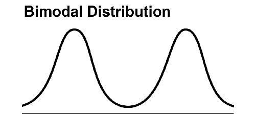
For example, a graph like this might show
the amount of money spent on lunches in a week (x-axis) and how many people spent that amount (y-axis). Imagine that you’ve got two different groups of people in your survey, children (left hump—they’re buying school lunches) and business executives (right hump—they’re going to fancy restaurants). The mean and median here could be a number somewhere right between the two, and would not tell us very much about what’s really going on—in fact, the mean and median in many cases are amounts that nobody spends. A graph like this is often a clue that there is heterogeneity in your sample, or that you are comparing apples and oranges. Better here is to report that it’s a bimodal distribution and report the two modes. Better yet, subdivide the group into two groups and provide statistics for each.
But be careful drawing conclusions about individuals and groups based on averages. The pitfalls here are so common that they have names: the ecological fallacy and the exception fallacy. The ecological fallacy occurs when we make inferences about an individual based on aggregate data (such as a group mean), and the exception fallacy occurs when we make inferences about a group based on knowledge of a few exceptional individuals.
For example, imagine two small towns, each with only one hundred people. Town A has ninety-nine people earning $80,000 a year, and one super-wealthy person who struck oil on her property, earning $5,000,000 a year. Town B has fifty people earning $100,000 a year and fifty people earning $140,000. The mean income of Town A is $129,200 and the mean income of Town B is $120,000. Although Town A has a higher mean income, in ninety-nine out of one hundred cases, any individual you select randomly from Town B will have a higher income than an individual selected randomly from Town A. The ecological fallacy is thinking that if you select someone at random from the group with the higher mean, that individual is likely to have a higher income. The neat thing is, in the examples above, that it’s not just the
mean
that is higher in Town B but also the
median
and the
mode.
(It doesn’t always work out that way.)
As another example, it has been suggested that wealthy individuals are more likely to vote Republican, but evidence shows that the wealthier states tend to vote Democratic. The wealth of those wealthier states may be skewed by a small percentage of super-wealthy individuals.
During the 2004 U.S. presidential election, the Republican candidate, George W. Bush, won the fifteen poorest states, and the Democratic candidate, John Kerry, won nine of the eleven wealthiest states. However, 62 percent of those with annual incomes over $200,000 voted for Bush, whereas only 36 percent of voters with annual incomes of $15,000 or less voted for Bush.
As an example of the exception fallacy, you may have read that Volvos are among the most reliable automobiles and so
you decide to buy one. On your way to the dealership, you pass a Volvo mechanic and find a parking lot full of Volvos in need of repair. If you change your mind about buying a Volvo based on seeing this, you’re using a relatively small number of exceptional cases to form an inference about the entire group. No one was claiming that Volvos never need repair, only that they’re less likely to in the aggregate. (Hence the ubiquitous cautionary note in advertising that “individual performance may vary.”) Note also that you’re being unduly influenced by this in another way: The one place that Volvos needing repair will be is at a Volvo mechanic. Your “base rate” has shifted, and you cannot consider this a random sample.